In what follows we will present examples of Deep Learning networks and detail their various designs. It is a detailed tutorial, written for students and engineers who want to acquire a profound understanding of the subject.
Concept of Depth in Deep learning
Deep Learning and the Universal Approximation Theorem
Shallow learning vs Deep learning vs very Deep learning
Shallow learning vs Deep learning
Deep learning vs Very Deep learning
Some Important concepts linked to deep learning
Connectionist temporal classification
CMAC (cerebellar model articulation controller)
Deep Boosting & Bootstrap aggregating
Credit Assignment Paths (CAPs)
Recursive Auto-Associative Memory (RAAM)
Neural Hierarchical Temporal Memory (HTM)
The Fundamental Deep Learning Problem
Feedforward (acyclic) vs recurrent (Cyclic) Neural Networks
Deep Learning and CPU & GPU power
Overview of the Increase in Neural Networks Complexity
Increase of neural network size
The Revolution of Deep Learning
Introduction
Deep learning is a recurring topic in the context of “Artificial Intelligence” but its definition is often unclear. Indeed, there are several different ways of understanding the concept as it groups a collection of notions and facts in Neural Networks.
In general Deep learning is connected with the idea of a ‘real’ Artificial Intelligence, in the sense that it achieves higher complexity than the average machine Learning algorithms for instance.
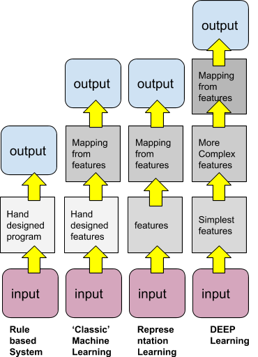
Deep Learning is often basically referred to as a multi-layered neural network but it has, in reality, the meaning of using multiple layers for processing different levels of features, from lower-level features to higher-level features, a bit like a pyramidal design of knowledge.
Deep Learning extracts information from one layer and passes it to the next layer and by doing so it can refine and reach a higher understanding of what is needed. Deep Learning is also connected with the important computation capacities of ‘modern’ CPUs which allow operating Neural Networks of the size of several millions of neurons. In fact, that computational power is maybe the most important aspects of Deep Learning rather than their designs so we could define Deep Learning in a simplistic way as such:
Deep Learning = Neural networks with many layers + progressive feature extraction and processing + CPU power + millions of neurons
In what follows we will try to present examples of Deep Learning networks and detail their various designs.
Generalities
As mentioned previously, there are many entry points for the understanding of what is Deep Learning. It can be seen as a way to learn the right representation for the data or to learn in a multi-step way.
In Deep learning, any layer of the representation can be seen as the analog of the state of the memory of a computer after the execution of another set of instructions in parallel.
Neural Networks which have a greater depth are able to execute more sequential instructions. Since they are able to execute instructions sequentially allows that next instructions can potentially use the results of previous instructions.
Following this, deep learning can be seen as neural networks where only a subset of the input representation for a given layer will be meaningful in terms of explaining and modeling the variations of that input. In deep learning, an input can be considered as the analog of a pointer for a computer program, eg an address which is in itself not representative of the data but which gives ways to the system to organize its processing.
According to many specialists in machine learning, deep learning is the only realistic approach for building A.I systems which can operate in complicated, real-world environments. Deep learning achieves great power and flexibility by learning to represent a real environment as a nested hierarchy of models, with each model defined in relation to simpler concepts.
Concept of Depth in Deep learning
Deep learning involves the idea of “depth” but this depth isn’t a rigorous mathematical concept here. While most approaches to deep learning consider the idea of a nested model - eg where features are progressively extracted and processed, from one layer to the next, the idea of depth varies and can be computed as the “length” of the flowchart needed to represent the computation or the number of times the model is being updated, which is of course relative.
Other computations of depth relate to ‘complexity’ notions, eg how much single concepts are needed. E.g., how much different concepts are needed to form the final neural net graph or flowchart.

For example, in the case of image recognition, the system can detect primitive shapes like circles (1) and then refine to detect eyes (2). This would mean a depth of two even if this involves more than 2 layers.
Deep Learning and the Universal Approximation Theorem
Deep learning is often associated with the Universal Approximation Theorem in neural networks. This theorem states that a feed-forward network containing only one hidden layer (with a finite number of neurons - hence a real neural network) can approximate any continuous function over compact sets of the n-dimensional real space , under weak assumptions on the activation function, mainly that it is not a polynomial.
One issue is that - to approximate functions - the width (not the ‘depth’) - of a neural network has usually to increase exponentially with the granularity required. There are several variants of that theorem including the approximation of Lebesgue-integrable functions by networks using re-Lu functions only.
What is important here is to understand that any - or almost any - sort of phenomenon can be approximated by neural nets, while their ability to be learned may be another story. But theoretically, neural nets have the capacity to represent a huge range of systems and our understanding is that the more complex the system is in terms of variations, the “deeper” the neural network must be.
Shallow learning vs Deep learning vs very Deep learning
Shallow learning vs Deep learning
The main characteristic of Deep Learning is that Deep Learning methods process and creates their own features directly from data (a.k.a ‘feature learning’), while Shallow Learning needs developers to write code to extract features based on rules and heuristics of the target problem.
Shallow learning represents the ‘classical’ machine learning approach. A special problem needs features to be extracted and rules to extract these features are developed by engineers outside the neural network while deep learning is able to learn the features and do not specific engineering for that.
Shallow learners are usually dependent on the features which have been engineered for creating the classification/prediction or regression model while, on the other hand, deep learners are potentially able to extract better features representation from the raw data in order to create much better models.
While deep learners models are much more generic (a bit like modern computer languages vs assembly code) and do not need the specific step of crafting the feature extraction, they are much more complex, much more demanding in terms of computer powers, they need much rawer data and therefore they are much harder to train efficiently. Opposingly to a shallow learner, a deep learner will have a great appetite for data and will very badly perform with sparse inputs!
As examples of shallow learners, we can cite for instance: decision trees, support vector machines (SVM), Naive Bayesian classifiers, etc...
As examples of deep learners, we can cite Multilayer feedforward neural networks, autoencoders, recurrent neural networks.
Deep learning vs Very Deep learning
Inside deep learning itself, there is a new restriction which involves the depth of the network. If the depth is >10 (and depth of a neural network is the relative measure itself) then the network may be considered to be a very deep learning network. The concept of very deep learning focus on the ideas that the very deep networks with skip (or residuals) connections are able to realistically reproduce recurrent computations - which would be similar to the recurrent connections in the visual cortex - or are actually exponential ensembles (fusion classifiers) of shallow networks.
There is no rigorous theory behind the very deep learning networks and it’s an actual area of debate when a network stops to be deep and becomes ‘very deep’.
Deep belief networks
Deep belief networks are linked to Deep learning. Deep belief networks (DBN) are probabilistic and generative multi-layered neural networks.
Generative modelling is a concept related to unsupervised machine learning - such as when the classifier needs to learn the features - as a way to describe real-world phenomena.
One can see Deep belief networks as a network of smaller learner units such as Boltzmann machines or AutoEncoders. (which are themselves neural nets) which could, therefore, be described as a “neural network” of neural networks.
A DBN is used in general to ‘pre-train’ a DNN by feeding the DNN initial weights as the weights which have been learned, making DNS an assistant or ‘pre-learning’ module of the DNN.
As we see these concepts involve already higher-level and more sophisticated and complex architectures than ‘traditional’ neural networks.
[See Deep Beliefs Networks article]
Deep Boltzmann machines
[see Boltzmann Machines article]
Some Important concepts linked to deep learning
We need to introduce some terms to be able to provide some facts about Deep Learning.
The following concepts are important for understanding deep learning architectures.
Neocognitron
The neocognitron has been conceived by Kunihiko Fukushima in 1979, as a hierarchical and multilayered neural network. It can be seen as a precursor of the convolution networks. The neocognitron is directly inspired by works that identified two types of cells in the primary visual cortex, simple cells, and complex cells. A simple cell in the primary visual cortex is a cell that responds primarily to oriented edges and gratings while Complex cells receive inputs from a number of simple cells. A complex cell behaves like a simple cell and will respond to oriented edges and gratings, but it also has special invariance properties and its receptive field cannot be mapped into fixed excitatory and inhibitory zones. Instead, a complex cell will only respond to specific patterns of light in a certain orientation regardless of the exact location. This means that these cells obey a hierarchical system that is replicated in the neocognitron.
The neocognitron is a natural extension of these cascading/ hierarchical models. The neocognitron consists of multiple types of cells: S-cells (a.k.a simple cells) and C-cells (a.k.a complex cells). The local features are first extracted by S-cells, and are later processed by C-cells, acting as local systems.
In neocognitron, the local features in the input are gradually processed and classified in the higher layers. This pyramidal, hierarchical, cascading processing is one of the bases of deep learning and can be found in networks such as the Convolutional Neural Networks, the SIFT method, and the HoG method.
Cresceptron
Cresceptron is based on a cascade of layers the same as the Neocognitron. But while Neocognitron needs a human programmer to craft the features extraction process, the Cresceptron is able to learn an open number of features in each layer in unsupervised learning mode. Each feature is being represented by a convolution kernel. Cresceptron can be described as one of the first deep Learning network, a self-organizing neural network which grows adaptively.
LSTM
The Long short-term memory network (LSTM) is an artificial recurrent neural network that is used in the area of deep learning. Since it is a recurrent network, LSTM has feedback connections therefore it can processes \'streams’ of data, continuous time-dependent sequences of data. LSTM are competitors of Markov Process-based classifiers and other similar time series classifiers.
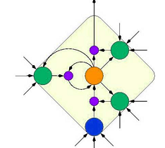
A typical LSTM unit is made up of a cell, an input and an output gate and a forget gate (‘keep gate’). The cell keeps in memory the values over the time intervals and the three gates control the flow of information into and out of the cell.
LSTM is a very important concept for building Deep Learning systems. They are used in non-trivial applications such as continuous handwriting recognition, speech recognition but also video games intelligent player bots, e.g bots which can actually play and win complex games such as Dota or Starcraft against humans.
Illustration: A typical LSTM cell
Connectionist temporal classification
The Connectionist temporal classification network (CTC) is a type of neural network used for the pre-learning phase in recurrent neural networks (RNNs) such as the LSTM networks.
CMAC (cerebellar model articulation controller)
The cerebellar model arithmetic computer (CMAC) - or equivalently the cerebellar model articulation controller - is a special type of neural network which is inspired by the biological cerebellum. It is also known as the. It is a type of associative memory. The biological cerebellum processes the information from the sensory nervous systems and other parts of the (biological) brain and then regulates the motor movements
The CMAC was initially proposed as a possible model for robotic controllers but it was introduced successfully in reinforcement learning and classifier for machine learning
The DCMAC - or Deep CMAC - stack several shallow structures and create a dep structure from them. It has been proved that this creates a better computing system. The deep CMAC is an important class of deep learning networks.
Deep Boosting & Bootstrap aggregating
Bootstrap aggregating which is also called ‘bagging’, is a fusion classifier 9ensemble classifier) which is designed to improve the accuracy and stability of machine learning algorithms in general. It can also be used to reduce overfitting. While Bagging is usually used with decision trees, it can be used with deep learning and has been proved to be an efficient booster for such networks.
Credit Assignment Paths (CAPs)
CAPs have been introduced as a measurement of whether learning in a given Neural network is of the deep or shallow type.CAP are chains of possible causal links between events.
Recursive Auto-Associative Memory (RAAM)
Deep Recursive Auto-Associative Memory or DRAAM is a recursive encoder and decoder network which can convert symbolic data to and from numerical vectors. RAAM will convert a list of symbols into a set of vectors - which will be dense (eg numerous, continuous-like) - and then uses an encoder to reduce their amount to a small discrete-like amount.
The decoder network on the other side will split a feature vector input until the input sentence embeddings are - approximately- recreated. This method shows how efficient are recursive neural networks when it comes to learning encodings for symbolic hierarchical data.
Neural Hierarchical Temporal Memory (HTM)
The Hierarchical temporal memory (HTM) is a concept biologically inspired by the physiology and organization of pyramidal neurons in the neocortex.
In HTM there are algorithms that are able to store information, learn and infer and remember complex temporal sequences. Same as LSTM, HTM learns a continuous time series flow of information in a completely unsupervised way. HTM is very robust to the noise inside input data and can learn continuously in parallel. It is used in applications that need anomaly detection like alert systems etc…
HTM and LSTM look similar but despite almost identical performances, HTM and LSTM process the data in two distinct ways: while LSTM requires many loops over data (since it is recurrent) for performing the learning and must compute the gradient- descent optimization algorithm each time, HTM only needs to process the data once.
Neural History Compressor
The neural history compressor is a stack of recurrent neural networks used in unsupervised learning.
Each input from a layer learns how to predict the output from the previous layer and therefore only unpredictable inputs are processed and forwarded to the next layer. Therefore the data are compressed between each layer to reach each time a higher level of compression. The initial input sequence can be reconstructed from the final output.
The neural history compressor has two different types of layers: the "conscious" chunker (higher level) and the "subconscious" automatizer (lower level)
Once the conscious chunker knows how to predict and therefore how to compress unpredictable inputs, they are sent to the automatizer, then the automatizer has to learn and predict or mimic.
The automatizer, therefore, will learn only what is needed to be learned since the conscious chunkers will rarely change.
Auto-Encoders (AE)
An autoencoder is a class of unsupervised neural networks used to learn efficient data codings. The autoencoder learns an encoding for a set of data, using dimensionality reduction, by training the network on how to remove noise.
Autoencoders compress input to a concise representation and then copy it to the output, reconstructing the compressed data. Autoencoders are basic bricks of a deep learning system, usually used for reducing the size of intermediary data.
This strategy has been applied to construct deep autoencoders to map images to short binary code for fast, content-based image retrieval, to encode documents (called semantic hashing), and to encode spectrogram-like speech features.
The Fundamental Deep Learning Problem
Deep neural networks are hard to train because they suffer from the now famous problem of vanishing or exploding gradients. There are several possible solutions to this:
- Unsupervised pre-training;
- LSTM-like networks;
- GPU-based computers a million times faster than when deep learning started, allowing for propagating errors a few layers further down within a reasonable time
- The space of Neural network weights can also be searched without using error gradients, and therefore avoiding the Fundamental Deep Learning Problem. In fact, some simple problems can use credit assignment (CAP) and random guesses.
Feedforward (acyclic) vs recurrent (Cyclic) Neural Networks
It is considered, in general, that feedforward neural networks have less ability to perform deep learning than recurrent neural networks.
[see the recurrent neural network section]
Deep Learning and CPU & GPU power
Deep learning is essentially made possible, concretely speaking, because of advances in hardware, especially in GPU chipsets.
Nvidia, the well-known graphic card manufacturer, was involved in what is considered as the ‘big bang’ of deep learning, 10 years ago since the deep learning units started to be trained with Graphical Processing Units from Nvidia.
GPUs and CUDA architecture is well-suited for linear computations such as matrix and vector computations, which are the base of neural networks.
Nvidia and other GPU chips manufacturers are even now producing deep learning compilers so that deep learning systems can be natively compiled for their GPU chips.
History of Deep Learning
In what follows we try to make a digest of the most significant events that led to deep learning development.
The Neocognitron introduced by Kunihiko Fukushima in 1980 is considered as the pioneering of deep learning.
In 1989, a team led by Yann LeCun used the standard backpropagation algorithm to train a deep neural network for recognizing handwritten numbers. While the algorithm worked, the training required 3 days.
The network used only 3 hidden layers but can be already considered as a deep learning network.
-2.png?width=609&name=pasted%20image%200%20(1)-2.png)
Yann LeCun and his colleagues will then develop further models, leading to the series of LeNet convolutional deep learning networks.
By 1991 such neural networks were used for recognition of 2D handwritten numbers, but the recognition of 3D objects was performed by matching 2D images with a manually designed 3D model.
This led to the development of the Cresceptron by Weng et al. The Cresceptron was able to naturally classify 3D objects as natural images.
Cresceptron started to use max-pooling and convolution kernels with the ability to extract features without a handcrafted model. Such architecture would become widely used in many different deep learning networks.
In 1994, André de Carvalho, Mike Fairhurst and David Bisset, developed a multi-layer boolean (weightless) neural network composed of a 3 layers self-organizing feature extraction module (SOFT) then followed by a classification module with multiple layers.
In 1995, Brendan Frey and colleagues developed the so-called wake-sleep algorithm which was able to train a network with six layers and several hundred hidden units. The networks suffered slowness especially because of the vanishing gradient problem (cf Fundamental problem of deep learning)
From 1990 to 2000 a simpler class of machine learning such as Gabor Filters or Support Vector Machines were preferred to deep learners. The reason was a clear lack of understanding of the mechanisms in the human brain that could inspire enough deep learning architectures.
In the field of speech recognition, most deep learning nets outperformed compared to other models such as the hidden Markov models classifiers for instance. There were a variety of reasons for this. Mainly the lack of computing power.
Nevertheless, some A.I/ML teams (Darpa, etc..) chose to develop deep learning systems and performed very well at several evaluations at the end of the ’90s.
Speech recognition was a playground from the ’90s for the deployment of deep learning, using inputs such as graphs of raw frequency banks over time or Mel-cepstral analysis, etc…
At the start of the 2000s, deep neural structures such as LSTM became competitive and were merged later with other networks such as connectionist temporal classification (CTC). More recently, in 2015, Google\'s speech recognition is supposed to have reached an important performance through CTC-trained LSTM.
In the mid-2000’s Deep beliefs networks started to appear. Deep neural systems were part of expert systems in computer vision, ASR, radar detection, etc…
The Convolutional neural networks (CNNs) were generally outperformed by CTC/LSTM but CNNs remained more successful in computer vision.
Industrial usage of neural networks started with CNNs such as leNet processing more than 20% of handwritten checks in the US for example.
In 2009, it was discovered that replacing pre-training with large data in certain contexts could make deep neural networks outperform largely their rivals, the Gaussian mixture model (GMM)/Hidden Markov Model (HMM).
Nevertheless, at the end of the 2000s and beginning of the ’10s, pre-training deep networks with deep belief networks are the de-facto norm for improvement of the deep learning models.
In the 10’s, advances in hardware have re-enabled interest in deep learning. In 2009, Nvidia created what is called a ‘big bang’ in deep learning by teaming with researchers - especially from google- to build GPU-based deep learning systems which could accelerate the computations by 100 times. Deep learning compilers and virtual machines are actively developed by graphical card manufacturer, parallelly to tensor processors, dedicated to “A.I”.
Overview of the Increase in Neural Networks Complexity
Datasets
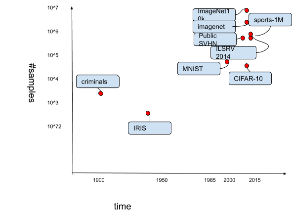
Next, we represent the development of deep learning through several visual representations,
First, we represent the increase of datasets used for training over time (logarithmic scale). The recent datasets such as ImageNet (over 14 million of samples) demonstrate the huge capacity for training deep learning networks.
Connection per neurons
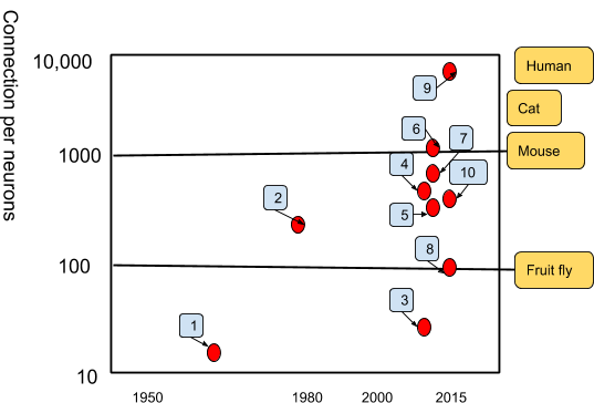
Here we represent how the connection between neurons has evolved, especially because of increases in hardware computations capacities. The latest neural networks reach levels comparable to the human brain (~ 10^4)
|
Number |
Neural network |
|
1 |
Adaptaline |
|
2 |
Neocognitron |
|
3 |
GPU-CNN |
|
4 |
Deep Boltzmann Machines |
|
5 |
Unsupervised CNN |
|
6 |
GPU multilayer perceptron |
|
7 |
Distributed Auto Encoder |
|
8 |
Multi-GPU CNN |
|
9 |
COTS HPC Unsupervised CNN |
|
10 |
GoogLenet |
Increase of neural network size
The next representation shows in a striking way how far have progressed the capacities of deep networks as they are compared to the capacity of brains of insects, invertebrates, mammals, and humans. At the present time, the size of a trained working deep neural network is to be compared to the brain of a bee.
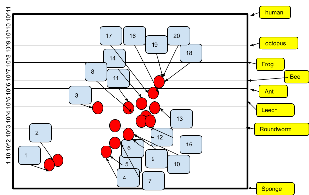
|
Number |
Neural network |
|
1 |
Perceptron |
|
2 |
Adaptaline |
|
3 |
Neocognitron |
|
4 |
Early backpropagation network |
|
5 |
Speech recognition RNN |
|
6 |
Speech recognition multilayer perceptron |
|
7 |
Mean Field sigmoid network |
|
8 |
LeNet-5 |
|
9 |
Echo State network |
|
10 |
Deep belief network |
|
11 |
GPU-CNN |
|
12 |
Deep Boltzmann Machines |
|
13 |
GPU Deep belief network |
|
14 |
Unsupervised CNN |
|
15 |
GPU multilayer perceptron |
|
16 |
OMP-1 network |
|
17 |
Distributed Auto Encoder |
|
18 |
Multi-GPU CNN |
|
19 |
COTS HPC Unsupervised CNN |
|
20 |
GoogLenet |
The Revolution of Deep Learning
We just looked at the surface of deep learning in this article. Deep learning induces a revolution in how we perceive (pseudo) Artificial Intelligence and Machine Learning because it allows us to create a synthetic intelligence that - in many ways - imitate and simulate the behavior of the brains of intelligent living organisms.
As we saw progress is very important, especially because hardware computational powers are growing day after day.
In terms of design and programming, Deep learning also creates a new world with complex designs involving modules made of subnets and so on…. This is maybe the more characteristic aspect of deep learning revolution: the ability to create neural nets that have the complexity of circuits designs for example. Regarding this, deep learning virtual machines and compilers are developed so that there could be a direct conversion between a neural net system and hardware in the same way compilers translate C# or C++ into bytecode or machine code.
Next to Deep Learning will probably see the rising of ‘very Deep learning’ but that is already another story.

